(DMAT, IMTech). Received on October 12, 2023.
The title of this lecture is a topic of the bachelor’s degree in Mathematics offered by the FME. There is a subject called Mathematical Models of Physics, which I have never taught, and which I am sure covers it much better than I will. But I will give my point of view. And my point of view is inspired, or wants to be inspired, by Newton’s Philosophiæ Naturalis Principia Mathematica. I need not explain to you that this is a very important book. In it Newton created mechanics, the three laws of mechanics; he created gravitation with the law of universal gravitation; and he created infinitesimal calculus, an extraordinary advance. And how did Newton proceed? He studied some problems and created the mathematics he needed. The mathematics he needed was the infinitesimal calculus and he created it. He was able to do it. I would like to look at the most typical fluid mechanics’ equations from this point of view, the point of view of the mathematics involved in those equations.
Linear algebra. Let me start with a central equation from Linear algebra:
![]()
Since I have never taught Linear Algebra, it is quite likely that Eq. (∗) is taught on the first day in that subject, I don’t know, but I do teach it on the first day. My proof of the formula uses the definition of the determinant by permutations. Indeed, all permutations except the identity produce terms in ε of order ⩾ 2, while the identity produces (1 + εa_{11}) · · · (1 + ε_{nn}) = 1 + ε(a_{11} + · · · + a_{nn}) + · · ·, where the last · · · denote terms of order ⩾ 2 in ε. And why do I say it is central? Because in the determinant on the left A may a Jacobian matrix and then second term, the trace, is a divergence.
This reasoning seems to go back to L. Euler (see [7]), but if we have to credit a name behind (∗), it has to be Jacobi, as he discovered a formula that is more general than (∗), but more complicated. Jacobi was an Ashkenazi Jew and I cannot refrain to quote Bell’s assessment found on borrowing his photograph below from Wikipedia: “Carl Gustav Jacob Jacobi was not only a great German mathematician but also considered by many as the most inspiring teacher of his time”. I do not use the term ‘inspiring’ in Catalan or Spanish, although I know who my ‘inspiring’ teachers have been and I am very grateful to them. If I wouldn’t know what ‘inspiring’ is, I surely know what it ends
up being.
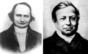
Carl Gustav Jacob Jacobi (1804-1851) and Joseph Liouville (1809-1882).
Differential equations. Liouville’s theorem for matrix solutions X(t) of ordinary linear homogeneous differential equations, X′(t) = M (t) ◦ X(t), can be stated as follows:
![]()
This is an easy consequence of the following relation and (∗) for ε = ∆t:
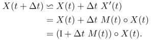
Indeed, these relations imply that
![]()
consequently
![]()
and the claim follows readily from this.
Liouville was (like Cauchy and like Navier) an engineer of “Ponts et Chaussées”, and also an engineer of the École Polytechnique. Apparently at that time mathematical analysis was taught at the École Polytechnique, and the teacher was Cauchy, while at the school of Ponts et Chaussées they made, well, bridges and roads. Let us keep this in mind for what we will say later.
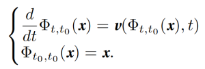
A little more complicated, but still in the subject of Differential Equations, is the problem of finding the derivative of an ordinary system of differential equations with respect to the initial conditions. This can phrased by means of the function Φ, called the flow of the equations, which it sends the initial condition at time t0 to the final condition at time t. The first formula below is the differential equation, and the second, the initial conditions:
Taking the derivative D with respect to x, we get
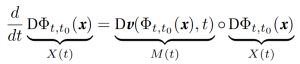
and by Louville’s theorem,
![]()
where JΦ = det(DΦ_{t,t0} (x)) is the Jacobian of the flux and Tr(Dv(Φ_{t,t0} (x0), t)) is the divergence of v. If the divergence is positive, the flow expands, and when it is negative, it contracts. Actually, this is the reason why ∇ · v is called ‘divergence’ of v.
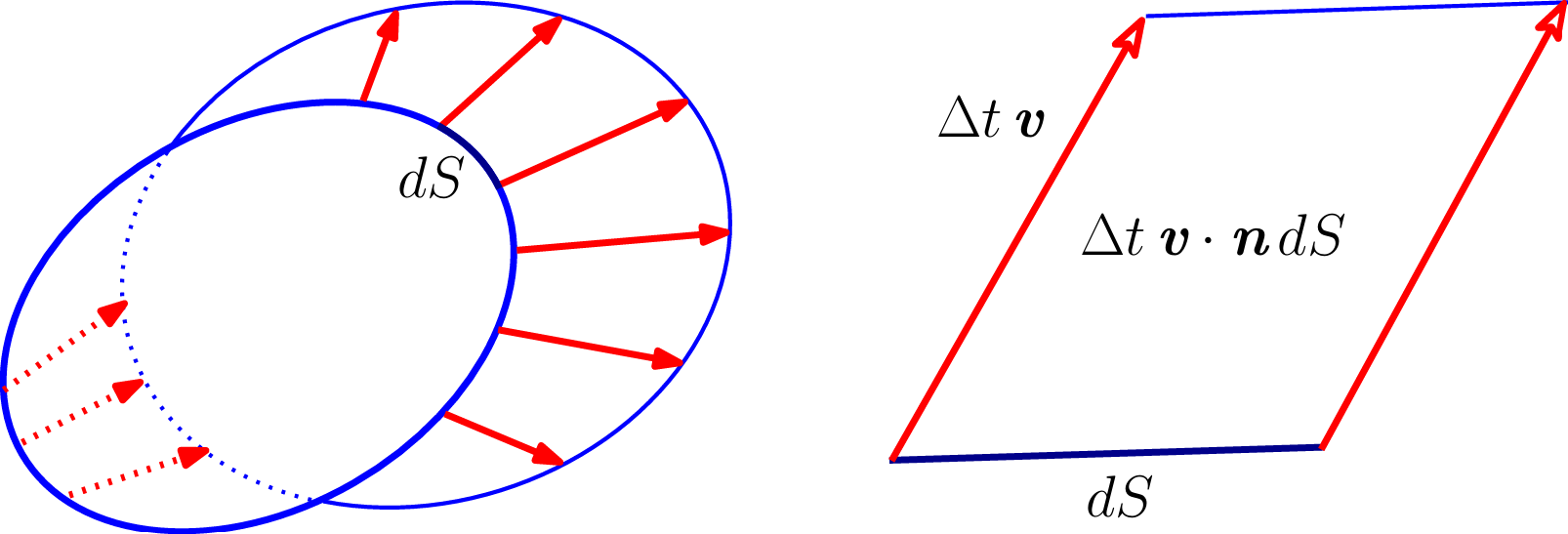
Integral calculus. The divergence theorem asserts the second equality in the following formulas:
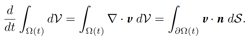
Let me look at those formulas in another way (for this view I recognize the influence of a former brilliant student I had, Joaquim Serra). For the first equality we use the change of variables formula![]() , for a fixed t0. Note that then the derivative with respect to t can be moved inside the integral and we have seen that the derivative of the Jacobian is the divergence. We can also consider what volume the border of Ω sweeps in its motion, which leads to the third formula: only the normal component of the velocity accounts for the change in volume (see next figure). In sum, we have two ways of calculating
, for a fixed t0. Note that then the derivative with respect to t can be moved inside the integral and we have seen that the derivative of the Jacobian is the divergence. We can also consider what volume the border of Ω sweeps in its motion, which leads to the third formula: only the normal component of the velocity accounts for the change in volume (see next figure). In sum, we have two ways of calculating![]() and therefore they yield the same result, which amounts to a proof of the divergence theorem.
and therefore they yield the same result, which amounts to a proof of the divergence theorem.
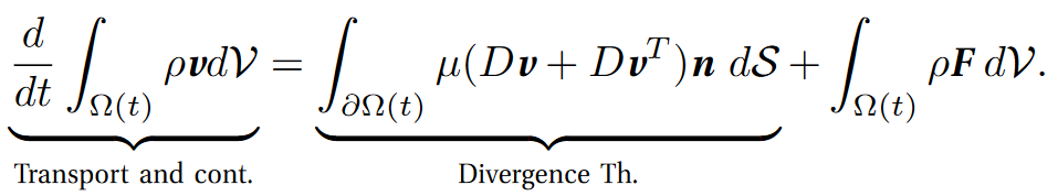
Reynolds’ transport theorem. Although it is possible to present fluid mechanics without recourse to this theorem, I am much in favor of its use. It asserts the following:

The left-hand side is again the derivative with respect to t of an integral over a domain moving with the flow, but now the integrand is not 1, as in the divergence theorem, but a general function f = f(x, t). In the integrand of the right-hand side we have the term ∂_{t}f (the variation of f with respect to t) and the divergence ∇ · (f v), which is equal to ∇f · v + f ∇ · v.
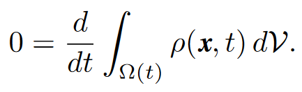
Conservation of mass and the continuity equation. Now we begin to look at fluid mechanics. The principle of conservation of mass is that the mass within any domain Ω() moving with the flow does not change. This can be expressed by asserting the vanishing of the derivative with respect to time of the integral of ρ(x, t) over Ω(t):
If we evaluate this derivative by means of Reynold’s transport theorem, we conclude that
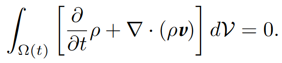
Since this happens for any domain, this relation is equivalent to
![]()
which is known as the continuity equation (for mass). In the case of an incompressible and homogeneous fluid, ρ = ρ0 (a constant) the continuity equation reduces to
![]()
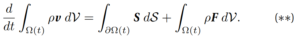
Balance of the linear momentum. The linear momentum of the mass ρ dV contained in the infinitesimal volume dV is ρv dV. Therefore the integral ![]() is the momentum of the mass contained in Ω(t). Its derivative with respect to t is the total force acting on Ω(t) (Newton’s second law). This total force is the sum of stress and body forces. The stress forces on the matter contained in Ω(t) are exerted by the matter outside the region through the boundary. They are represented by the vector S (force per unit boundary area) and hence the total stress force is given by the integral
is the momentum of the mass contained in Ω(t). Its derivative with respect to t is the total force acting on Ω(t) (Newton’s second law). This total force is the sum of stress and body forces. The stress forces on the matter contained in Ω(t) are exerted by the matter outside the region through the boundary. They are represented by the vector S (force per unit boundary area) and hence the total stress force is given by the integral ![]() . The body forces are represented by the vector F that encodes the force per unit mass, so that the total of such forces on Ω(t) is
. The body forces are represented by the vector F that encodes the force per unit mass, so that the total of such forces on Ω(t) is ![]() . Gravity and Coriolis forces are of this kind. In sum, the balance of linear momentum for a fluid is expressed by the equation
. Gravity and Coriolis forces are of this kind. In sum, the balance of linear momentum for a fluid is expressed by the equation
Leonhard Euler (1707 – 1783)
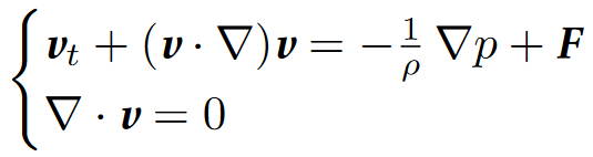
Euler’s equations for incompressible non-viscous fluids. For non-viscous fluids, the stress forces are necessarily normal to the boundary: S = −pn (this is analogous to the fact that a perfectly slippery surface can only react with normal forces to any object touching them). The scalar p is called pressure. Using the divergence theorem, it can be seen, as in [2], that the total stress force can be expressed as a volume integral: ![]() . In this case the balance of momentum gives, using the transport theorem for each component ρv^{i} of ρv (i = 1, 2, 3),
. In this case the balance of momentum gives, using the transport theorem for each component ρv^{i} of ρv (i = 1, 2, 3),
![]()
which, using the continuity equation, yields Euler’s equations (1757) for an incompressible non-viscous fluid:
In the PDEs course taught in our curriculum these equations are only studied in a much simpler version, namely Burger’s equation: u_{t} + uu_{x} = 0. Here the unknown u is a scalar, not a vector. The term uu_{x} = (u∂_{x})u corresponds to (v · ∇)v, and there are no terms corresponding to the gradient of the pressure nor the equation analogous of ∇ · v = 0.
PDEs. Euler’s equations have a remarkable connection with Laplace’s equation ∆ϕ = 0. If we assume that v(x, t) = v(x) = ∇ϕ (in this case we say that v is a potential flow), the condition ∇ · v = 0 becomes ∇^{2}ϕ = ∆ϕ = 0 and Euler’s equations are satisfied with p = − (1/2) · ρ∥v∥^2 + C (this is Bernoulli’s equation, which is also valid for irrotational flows). Two significant propertis of potential flows (see [2]) are that, on one hand, their circulation around any closed curve is zero, and, on the other, that they minimize the kinetic energy among all flows that satisfy the same (Neumann) boundary conditions (i.e., imposing the value of the normal derivative at a boundary).
If a field is the gradient of a function, its rotational is zero. The converse is true only when the domain of the field is simply-connected (a topological condition).
Another remark is that the wave equation
![]()
can also be regarded as a fluid mechanics equation, but this time for compressible flows (p = p(ρ)). Indeed, in this case it turns out to be a consequence of Euler’s equation for potential flows (see [1]).
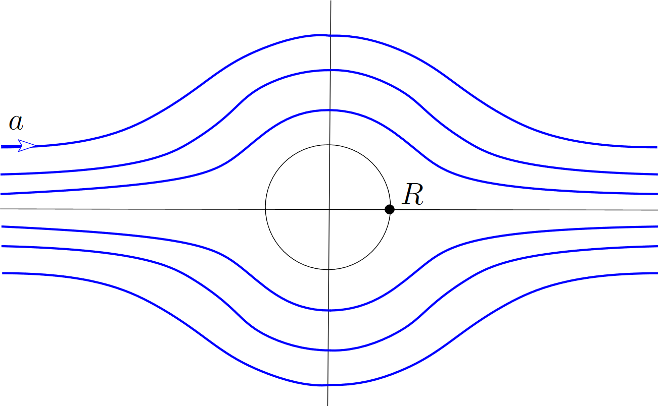
Complex analysis. In Complex analysis (one of the subjects of our Mathematics curriculum), it is proved that the harmonic functions are the real part of holomorphic functions in simply-connected domains. If this is the case, a complex potential Ω(z) = ϕ(x, y) + iψ(x, y) is introduced, where ϕ(x, y) is the velocity potential. Now the Cauchy-Riemann conditions imply that the integral curves of v are the level curves of ψ(x, y) (i.e., the curves ψ(x, y) = constant). For example, level curves corresponding to the imaginary part of the function Ω(z) = a(z + R^{2}/z), which is holomophic outside the disc of radius R, are depicted in the following picture, where a is the velocity at infinity:
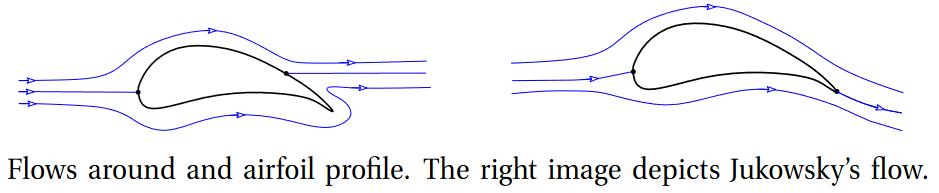
However, potential flows around an obstacle are cursed by the D’Alembert’s paradox (in dimensions 2 and 3): Such flows, with given velocity at infinity, do not produce any net force on the obstacle.
An important breakthrough for curing that paradox was discovered by Nikolai ZhukovskyW (1847-1921). He was a Russian scientist who is considered a founding father of hydrodynamics and aeronautical engineering. In his research of how a flow could produce a lifting force on a plane wing profile, he took recourse in his knowledge of complex analysis, including the technique of computing integrals by means or residues, and thereby he modified the complex flow considered before by adding a term ![]() (this term is irrotational, but not potential, inasmuch as the exterior of the profile is not simply-connected). The net result is that it produces a lift force with no drag.
(this term is irrotational, but not potential, inasmuch as the exterior of the profile is not simply-connected). The net result is that it produces a lift force with no drag.
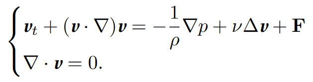
Viscous flows: Navier–Stokes equations. Drag is produced by viscosity, which is reflected in the form of the stress vector S. Cauchy showed that S = σ · n, where σ is a symmetric matrix (it is called Cauchy’s stress tensor). It follows that we can write σ = −pI + σ_{v}, where σv is also a symmetric tensor. This tensor is called the viscosity tensor as σv = 0 precisely when the flow is non-viscous (that is, σ = −pI).
The fundamental fact about the viscosity tensor is that σ_{v} depends linearly on the differences of velocity between nearby particles (Navier, Stokes). Therefore it is reasonable to write σ_{v} = σ_{v}(Dv), where Dv stands for the differential of v, because Dv is a good encoding of the ‘velocity differences between nearby particles’. An additional remark is that the differences in velocity among nearby particles produced by rigid rotations do not produce viscous effect, and so we can replace Dv by Dv + Dv_{T} . By using (∗∗), it can be seen, as in [1, 2], that the result is the Navier-Stokes equations (NS), where μ is the fluid viscosity:
These equations lead to the standard form, with ν = μ/ρ (kinematic viscosity):
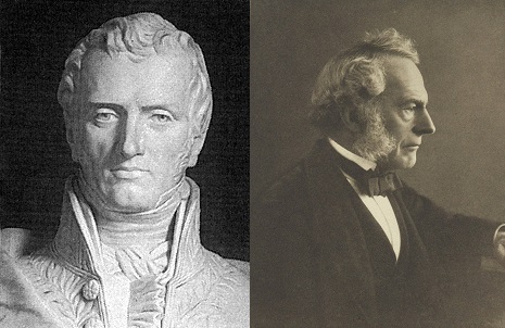
Claude-Louis Navier (1785 – 1836) and Sir George Stokes (1819 –1903)
The history of the NS equation is fascinating. As stated in [3], “Navier’s original proof of 1822 was not influential, and the equation was rediscovered or re-derived at least four times, by Cauchy in 1823, by Poisson in 1829, by Saint-Venant in 1837, and by Stokes in 1845. Each new discoverer either ignored or denigrated his predecessors’ contribution. Each had his own way to justify the equation. Each judged differently the kind of motion and the nature of the system to which it applied”. Cauchy and Poisson espoused the more mathematical approached, but otherwise their methodologies were quite different: Cauchy introduced tensor techniques and spatial symmetry arguments and Poisson, among other things, emphasized the need of molecular reasoning (discrete sums instead of integrals), as Navier had already pioneered. Saint-Venant and Stokes acknowledged Navier’s work, but differed from him, and among themselves, on the procedures to get the equations.
So, why did the equations end up being called after Navier and Stokes? This question has been discussed in the history texts (see [3, 4], [5], [6], for example). One fact that is recognized is that Navier and Stokes were the most practical, the ones who cared more about contrasting their results with experiments, whereas the other names referred to above cared more about geometry. Navier, who died in 1836, remained a little skeptical about his equations because the experiments carried out by Girard, a professor at the École Polytechnique, did not quite turn out the way he expected. After his death, Hagen and Poiseulle designed more careful versions of Girard’s experiments and they found a better accord between theory predictions and experiments. As expressed in [3], it was unfortunate for Navier to trust Girard’s findings about flows in capillary tubes.
Stokes was also concerned with experiments. One important problem he studied was the drag F of a sphere moving inside a fluid. He came up with a formula named after him: F = 6πμRv, where R is the radius of the sphere and v the flow speed. I wish I had time to spend explaining where this formula comes from, and how many assumptions have to be made to get there. This formula is only valid in dimension 3. For the problem in dimension 2, that is, the movement of a disc in a plane fluid, or of a cylinder in a three-dimensional fluid, Stokes did not find a solution, and this is why it has remained as Stokes’ paradox. Now we know, as it was found out later, that there is no solution in dimension 2 (this would be a topic for another occasion). Stokes also introduced singular limits: his formula holds for a small sphere in very slow motion in a very viscous fluid.
A new derivation of the viscous term. The derivation I propose of the term μ∆v is based on the following formula:
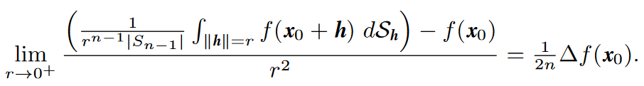
I learned this formula, which is not very well known, from Xavier Cabré. The term within parenthesis in the numerator is the average f_{x0,r} of the function f over the sphere of radius r centered at x0, i.e. the integral of the function over the sphere divided by the sphere’s area. The formula thus says that the value of the Laplacian of f at a point x0, ∆f (x0), can be obtained (note the factor 1/2n) from the limit when r → 0+ of the difference ![]() divided by r^{2}.
divided by r^{2}.
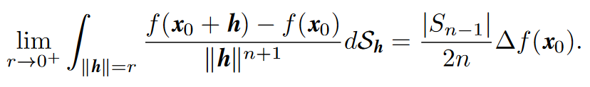
In the formula the function f can be vector valued and hence it can be applied to a flow v. In this case, the left hand side takes into account the difference![]() , which is a measure of the difference in a speed of the flow at a distance r from x0 and at x0. This view of the viscosity term goes to the root of the viscosity phenomenon: viscosity is produced by differences in speed between nearby particles, where ‘nearby’ means for ‘small’ r, that is, for r → 0+. It sheds a different light on the nature of the viscosity term included in the presentations by Navier, Cauchy, Poisson, Saint-Venant and Sokes. Whereas these authors derive the viscosity term by means of differential calculus, the proposed presentation relies on integral calculus.
, which is a measure of the difference in a speed of the flow at a distance r from x0 and at x0. This view of the viscosity term goes to the root of the viscosity phenomenon: viscosity is produced by differences in speed between nearby particles, where ‘nearby’ means for ‘small’ r, that is, for r → 0+. It sheds a different light on the nature of the viscosity term included in the presentations by Navier, Cauchy, Poisson, Saint-Venant and Sokes. Whereas these authors derive the viscosity term by means of differential calculus, the proposed presentation relies on integral calculus.
On the fractional Laplacian and Stokes’ paradox. To conclude, I am going to propose a similar approach to justify the use of the fractional Laplacian in the NS equations, as in [8, 9], a point that is hard to find, if at all, in the literature.
The following formula is the same as the preceding one, but written by moving f (x0) within the integral and |Sn−1| to the right-hand side:
Next formula has a similar look, and it is also the limit of an integral average, but it is different, as the integration runs over the exterior of the sphere of radius r.
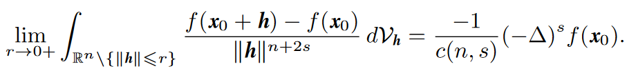
It is another way of construing the notion of velocity differences between nearby particles, and on the right hand side we get the fractional laplacian (−∆)^s. With this interpretation we obtain the NS equation with viscosity term expressed as a fractional Laplacian:
![]()
None of the central problems of the NS equations has been solved with this new equation, but one that I think has not been studied is this little nugget for which I have some sympathy: the Stokes paradox. Such study might produce, in dimension 2, an explicit solution to the flow problem around a disk. In other words, the question (perhaps open) is whether for some values of s in the fractional Laplacian there is no Stokes paradox in dimension 2, and thereby spawning an explicit solution for the flow around a disc.
References
[1] S. C. Hunter, Mechanics of Continuous Media, Ellis Horwood, 1976.
[2] A. J. Chorin and J. E. Marsden, A Mathematical Introduction to Fluid Mechanics, Springer-Verlag, 1979.
[3] O. Darrigol, Between hydrodynamics and elasticity theory: The first five births of the Navier-Stokes equation, Arch. Hist. Exact Sci. 56 (2002), 95-150.
[4] ___, Worlds of Flow: A Hystory of Hydrodynamics From the Bernoullis to Prandtl, Oxford University Press, 2005.
[5] X. Mora, Les equacions de Navier-Stokes. Un repte al determinisme newtonià, Butlletí de la Societat Catalana de Matemàtiques 23 (2008), no. 1, 53–120.
[6] S. R.Bistafa, On the developementof the Navier-Stokes equations by Navier, Revista Brasileira de Ensino de Física 40 (2018), no. 2, e2603.
[7] J. Cufí and A. Reventós, A historical review of the Cauchy-Riemann equations and the Cauchy Theorem, 2023. Preprint (41 pages), Dept. of Mathematics, UAB.
[8] Zhi-Min Chen, Analytic Semigroup Approach to Generalized Navier-Stokes Flows in Besov Spaces, Journal of Mathematical Fluid Mechanics 19 (2017), no. 4, 709-724.
[9] T. Dlotko, Navier–Stokes Equation and its Fractional Approximations, Applied Mathematics and Optimization 77 (2018), 99–128.