
Josep Masdemont (DMAT, IMTech)

The collinear equilibrium points of the Restricted Three-Body Problem (RTBP) were first described by the Swiss mathematician Leonhard Euler in the 18th century. The foundational understanding of libration point orbits has its roots in the pioneering work on the continuation of periodic orbits by Hénon and others laid the groundwork for both theoretical advances and practical applications culminating in the ISEE-3 mission in 1978—the first spacecraft to exploit the dynamical properties of the \(L_1\) point in the Sun–Earth system.
The success of ISEE-3 and the recognition of libration point orbits (LPOs) as privileged locations for solar and astronomical observation led to a series of landmark missions that demonstrated the value of these regions. Halo and Lissajous orbits around \(L_1\) and \(L_2\) have since been employed in numerous missions, including SOHO, Herschel, Planck, ARTEMIS, Gaia, Chang’e 2, Queqiao, Euclid, and the James Webb Space Telescope, offering favorable geometry for both scientific operations and continuous Earth communication.
Geometrically, the dynamics near collinear equilibrium points are governed by the structure of invariant manifolds, which are normally hyperbolic, and whose stable and unstable components act as phase space conduits. These structures determine the local behaviour, organize transfers between different orbits and facilitate the design of low-energy trajectories close to heteroclinic and homoclinic connections. The intersection of invariant manifolds between different LPOs provides the framework for natural transfer trajectories with minimal control effort. When exact connections are not available due to energy mismatch or mission constraints, such transfers can be enhanced through carefully designed maneuvers.
The Restricted Three-Body Problem (RTBP) is the classical model in celestial mechanics describing the motion of an infinitesimal mass under the gravitational influence of two massive primaries \(M\) and \(m\) (\(M\ge m\)). In the usual synodical reference frame they have the form, where \(\mu \in (0, 1/2]\) denotes the dimensionless mass parameter \(\mu = m / (M + m)\). The RTBP can formulated in Hamiltonian form with Hamiltonian \(H(x,y,z,p_x,p_y,p_z)\),
$$
H = \frac{1}{2}(p_x^2 + p_y^2 + p_z^2) + y p_x – x p_y – \frac{1 – \mu}{r_1} – \frac{\mu}{r_2}
-\frac{\mu}{2}(1-\mu).
$$
where \(r_1\), \(r_2\) are the distances to the primaries.
The RTBP has five equilibrium points, known as the libration points, where the gravitational and inertial forces balance. Three of them, denoted by \( L_1, L_2, L_3 \), lie on the line connecting the two primaries and are called collinear libration points. The remaining two, \( L_4 \) and \( L_5 \), form equilateral triangles with the primaries.
The collinear points are located along the \( x \)-axis in the synodical frame and their position are determined by the so called Euler’s quintic equations. Their local dynamics is described by the second order part of the Hamiltonian, \(H_2\) which admits a symplectic change of coordinates wich puts it in the normal form,
\begin{equation}\label{eq:H2}
H_2(\boldsymbol{q},\boldsymbol{p})=\lambda_0 q_1p_1+\frac{\omega_0}{2}\bigl(q_2^{2}+p_2^{2}\bigr)+\frac{\nu_0}{2}\bigl(q_3^{2}+p_3^{2}\bigr), \;\;\;\; (8)
\end{equation}
where \(\boldsymbol{q}=(q_1,q_2,q_3)\), and \(\boldsymbol{p}=(p_1,p_2,p_3)\) are generalized positions and momenta. So the linear flow has a center\(\times\)center\(\times\)saddle structure. The two purely imaginary eigenvalue pairs are linked to center-type motions. The center directions associated with \(\omega_0\) lies in the \((x,y)\) RTBP plane and gives rise to oscillations associated with the planar Lyapunov family; the other corresponds to oscillations in the \(z\) direction and originates the vertical Lyapunov family. The existence of these continuous families of periodic orbits in the nonlinear system is guaranteed by the Lyapunov center theorem.
The center manifold constitutes an example of what is called a normally hyperbolic invariant manifold. The dynamics of (8), is topologically equivalent to the full RTBP nonlinear system in a limited neighborhood \({\cal R}\) of the libration point. Considering a small fixed value of the Hamiltonian \(H_2=h\),
$$
R(h)=\Bigl\{(\boldsymbol{q},\boldsymbol{p})\in\mathbb{R}^6 \;\Big|\;
H_2(\boldsymbol{q},\boldsymbol{p})=h,\;
\lvert q_1-p_1\rvert\le K_{h}\Bigr\}.
$$
The first condition fixes the energy, reducing the six–dimensional phase space to the five–dimensional energy surface \(\{H_2=h\}\). The second condition bounds the equilibrium region in the \((q_1,p_1)\)–plane.
The condition \(H_2=h\) can be written as
$$
\frac{\omega_0}{2}(q_2^2 + p_2^2) + \frac{\nu_0}{2}(q_3^2 + p_3^2) + \frac{\lambda_0}{4}(q_1 + p_1)^2 = h + \frac{\lambda_0}{4}(q_1 – p_1)^2
$$
which means that \(R(h)\) is homeomorphic to \(S^4\times I_h\) where the interval \(I_h=[-K_h,K_h]\).
Taking into account that \(q_1p_1\), is a first integral, for each point in the \((q_1, p_1)\)-space, the set
$$
S^3_h(q_1,p_1)=\left\{
\frac{\omega_0}{2}(q_2^2 + p_2^2) + \frac{\nu_0}{2}(q_3^2 + p_3^2)=h-\lambda_0\,q_1p_1
\right\}
$$
is a \(S^3\) sphere parameterized by the center coordinates \((q_2,p_2,q_3,p_3)\). Because \(q_2^2+p_2^2\) and \(q_3^2+p_3^2\) are also first integrals, the energy \(h\) is split in the tree modes (the planar and vertical oscillations and the sadlle), when \(q_2=p_2=p_3=p_3=0\) we find that the hyperbolas \(q_1p_1=h/\lambda_0\) bound \(R(h)\) in the \((q_1,p_1)\) projection, and in these hyperbolas the corresponding \(S^3_h\) spheres become a point (see Fig. 8). Beyond the hyperbolas we have regions energetically forbidden (filled in salmon in the figure). Moreover, the condition \(\lvert q_1-p_1\rvert\le K_{h}\) creates two line segments \(p_1=q_1\pm K_h\) denoted by \(l_1\) and \(l_2\) which also bound \(R(h)\) in the \((q_1,p_1)\) projection (pale green region). The area to the left of \(l_1\) and the one to the right of \(l_2\) correspond to different realm regions (interior or exterior, to the realm of a primary, depending on the L\(_i\)).

Due to \(q_1p_1\) is a first integral, the orbits display an hyperbolic motion on the \((q_1,p_1)\) projection. Of particular interest is the case \(q_1p_1=0\) with the subset \(q_1=p_1=0\), defining the \(S^3\) sphere of central manifold trajectories at energy \(h\) (central black dot in Fig. 8); \(p_1=0\), \(q_1\ne 0\) defining its center-unstable manifold and \(q_1\ne 0\), \(p_1=0\) the center-stable ones (both displayed in green). Trajectories with \(q_1p_1 \ge 0\) correspond to transit orbits from one region to the other (displayed in red) while the ones with \(q_1p_1 \le 0\) correspond to non transit orbits (displayed in blue) [3].
When dealing with the full nonlinear problem, considering complex variables and Lie series transformations, one can obtain a truncated normal form at high order that gives \(\boldsymbol{q}_1(t)=\boldsymbol{p}_1(t)=0\) for all \(t\), provided that \(\boldsymbol{q}_1(0)=\boldsymbol{p}_1(0)=0\). This invariance condition assures that an orbit with \(\boldsymbol{q}_1(0)=\boldsymbol{p}_1(0)=0\) remains in the center manifold. Different normal forms, or partially normal forms, can be considered to fulfill the invariance condition. A usual one is the Birkhoff normal form which defines actions \(I_i={q}_i{p}_i\), \(i=1,2,3\), and then,
$$
H({\boldsymbol{q}}, {\boldsymbol{p}}) = H_2({\boldsymbol{q}}, {\boldsymbol{p}}) +\!\!\!\!\!\!\!\sum_{3\le i+j+k \le n }\!\!\!\!\!\!\! h_{ijk}\,I_1^i I_2^j I_3^k + R_n({\boldsymbol{q}}, {\boldsymbol{p}}).
$$
The truncated normal form is obtained removing the remainder \(R_n({\boldsymbol{q}}, {\boldsymbol{p}})\) [4].

A Hamiltonian fulfilling the invariance condition is useful to understand and visualize the whole dynamics in the center manifold. Roughly speaking, the Hamiltonian is reduced to the center manifold setting \({q}_1={p}_1=0\) which avoids the instability, so long-term numerical integrations are possible with the reduced Hamiltonian \(\widehat{H}({q}_2,{p}_2,{q}_3,{p}_3)\). We select the Poincaré section \(\{{q}_3=0\}\) and a fixed value \(\widehat{h}\) of the Hamiltonian \(\widehat{H}\). The intersection of the constant–energy three-dimensional manifold \(\{\widehat{H}=\widehat{h}\}\) with the section \(\{{q}_3=0\}\) is two–dimensional and can therefore be represented in the \(({q}_2,{p}_2)\)–plane. Given \(\widehat{h}\) we choose an initial \(({q}_2,{p}_2)\) pair and solve numerically the constraint \(\widehat{H}({q}_2,{p}_2;{q}_3=0,{p}_3)=\widehat{h}\) for \({p}_3>0\) (two opposite sign roots exist, of which we keep the positive one), and integrate the reduced Hamiltonian equations forward in time. Each subsequent crossing of the trajectory with \({q}_3=0\) and \({p}_3>0\) is plotted, producing a stroboscopic portrait of the phase space at the chosen energy (see Fig. 9).
Heteroclinic or homoclinic trajectories associated to libration point orbits provide natural transfer paths at zero propulsive cost. Such orbits are of interest in the trajectory design of missions like the NASA missions Genesis (Sun-Earth case) or Artemis (Earth-Moon case).
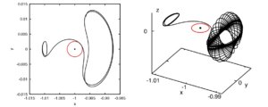
A simple way to introduce the concept is through periodic orbits in the planar RTBP. In the local neighbourhood of a collinear equilibrium point, and for an energy level close to that of the equilibrium, there is only one periodic orbit. A typical example is given by heteroclinic orbits linking planar Lyapunov orbits around \(L_1\) and \(L_2\) in the Sun-Earth problem.
The main procedure to detect such connections begins by defining a suitable surface of section \(\mathcal{S}\). The stable and unstable manifolds of the reference periodic orbits are then numerically integrated and their intersections with \(\mathcal{S}\) are recorded. In the simplest consideration, one obtains closed curves and their intersections give heteroclinic trajectories, due to the fact that the planar restriction is a two degrees of freedom Hamiltonian where obits and manifolds are in the same energy level.
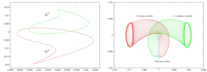
In the 3D case, and again for a fixed Jacobi constant of the RTBP, the propagation of the manifolds to \(\mathcal{S}\) produces \(S^3\)-spheres, so their transversal intersection inside \(\mathbb{R}^4\) (the six dimensional space is constrained by energy and section \(S\)) topologically is an \(S^2\)-sphere instead of a finite set of points.
It is worth noting that the \(S^2\)–sphere family of heteroclinic connections does not occur entirely between the same pair of 2D tori (i.e., the same Lissajous orbits), but rather spans a range of them. The stable manifold of a given Lissajous orbit connects heteroclinically to a set of Lissajous orbits on the opposite side, and in the case of homoclinic connections (understood here as homoclinic to the region, not to a single orbit), to a range of tori in its vicinity. This structure provides a clear example of Arnold diffusion mechanisms within \(W^c\) [2].
Most studies exploit the classical RTBP, taking advantages of its autonomous characteristics. However, Earth–Moon RTBP neglects the Sun’s direct gravity influence on the spacecraft and indirect influence on the Earth and Moon. As the missions become more complicated, higher fidelity non-autonomous four-body problems become more necessary. The Bicircular Problem, Quasi-bicircular Problem (QBCP), and Hill Restricted Four-Body Problem are the most extensively studied models, they are all periodic-pertubated systems. The QBCP considers the Sun, Earth and Moon in a solution of the general planar three-body problem and one can consider Sun-Earth Moon perturbed or Sun-Earth to Earth-Moon heteroclinics.
However computing tori and their manifolds in non-autonomous system is more complex than in autonomous system because the problem adds the set of frequency perturbations of the non-autonomous one. 2D invariant tori in CRTBP become 3D invariant tori in QBCP. In these settings, an additional difficulty appears: the stable and unstable manifolds must intersect at the same phase of the Sun–Earth–Moon system.
The quasi-bicircular problem is a planar approximation for the real Sun–Earth–Moon–spacecraft four-body system. It considers the primaries revolve in planar quasi-bicircular periodic trajectories of the general three-body problem. the dynamics of a massless fourth particle \(P\), is expressed in two synodical reference frames, the Sun–barycenter \(S^{SE}\) and the Earth–Moon \(S^{EM}\). Both formulations share the same formal expression for the Hamiltonian,
$$
\begin{aligned}
H(\boldsymbol{x}, \theta) =
& \frac{1}{2} \alpha_1(t) \left(p_x^2 + p_y^2 + p_z^2\right) + \\
& \alpha_2(t) \left(p_x x + p_y y + p_z z\right) + \alpha_4(t) x + \\
& \alpha_3(t) \left(p_x y – p_y x\right) + \alpha_5(t) y – \\
& \alpha_6(t) \sum \limits_{b \in \mathbb{B}} \frac{m_b}{\left\| \boldsymbol{r} – \boldsymbol{q}_b(t) \right\|},
\end{aligned}
% \label{eq:qbcp_senc_ham}
$$
where \(\alpha_i(t)\), are \(T\)-periodic coefficients, \(\mathbb{B} = \{\text{S}, \text{E}, \text{M}\}\) denotes the set of primaries (Sun, Earth, Moon) and \(\boldsymbol{q}_b(t)\) their corresponding position vectors.
The parameterization method is one way to represent invariant manifolds associated with invariant objects by means of high-order expansions [6]. For periodic non-autonomous systems, the manifolds associated to \(L_i\) dynamical equivalents (resonant periodic orbits) are parameterized in Fourier–Taylor series [1]. The method constructs a conjugacy between an \(n\)-dimensional invariant manifold \(\mathcal{M} \subset C^n\) of the \(T\)-periodic vector field \(\dot{\boldsymbol{z}}=\boldsymbol{F}(\boldsymbol{z},t)\) and a lower-dimensional model manifold \(\mathcal{S}\) with coordinates \(\hat{\boldsymbol{s}} \in \mathbb{C}^d\), governed by a reduced vector field \(\dot{{\boldsymbol{s}}}={\boldsymbol{g}}({\boldsymbol{s}},t)\). The manifold \(\mathcal{M}\) is parameterized by a map \(\boldsymbol{z}={\boldsymbol{w}}({\boldsymbol{s}},t)\), which is obtained by means of the invariance equation
$$
\boldsymbol{F}({\boldsymbol{w}}({\boldsymbol{s}},t),t) = \frac{\partial {\boldsymbol{w}}(\boldsymbol{s},t)}{\partial {{\boldsymbol{s}}}} {\boldsymbol{g}}({\boldsymbol{s}},t) + \frac{\partial \boldsymbol{w}( \boldsymbol{s},t)}{\partial {t}}.
$$
Both, the parameterization \({\boldsymbol{w}}\) and the reduced dynamics \({\boldsymbol{g}}\), are recursively computed and expressed by truncated multivariate Fourier–Taylor expansions,
$$
{w}_p({\boldsymbol{s}}, t)=\sum_{k=0}^{K}\sum_{\boldsymbol{r}\in\mathcal{R}_k}\sum_{j=-J}^{J} {w}_{p}^{\boldsymbol{r},j}\,e^{\text{i} j\omega t}\,{\boldsymbol{s}}^{\boldsymbol{r}}+\mathcal{O}(|{\boldsymbol{s}}|^{K+1}),
\label{eq:pm_w}
$$
$$
{g}_p({\boldsymbol{s}}, t)=\sum_{k=0}^{K}\sum_{\boldsymbol{r}\in\mathcal{R}_k}\sum_{j=-J}^{J} {g}_{p}^{\boldsymbol{r},j}\,e^{\text{i} j\omega t}\,{\boldsymbol{s}}^{\boldsymbol{r}}+\mathcal{O}(|{\boldsymbol{s}}|^{K+1}),
$$
where \(\boldsymbol{r}\) is a multi-index and \(\mathcal{R}_k=\{\boldsymbol{r}\in\mathbb{N}^d:|\boldsymbol{r}|=k\}\).
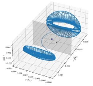
Using the parameterization method one can obtain accurate local representations of libration point orbits and their manifolds which can be propagated by numerical methods. The heteroclinic connections between the \(L_1\) and \(L_2\) orbits of the Sun–Earth system can be strongly perturbed when the Moon is included in the model. As a result, it becomes possible to obtain connections between orbits with very different amplitudes [5] (see Fig. 10).
References
[1] B. Le Bihan, J.J. Masdemont, G. Gómez, and S. Lizy-Destrez. Invariant manifolds of a non-autonomous quasi-bicircular problem computed via the parameterization method. Nonlinearity, 30:3040–3075, 2017. DOI 10.1088/1361-6544/aa7737.
[2] A. Delshams, M. Gidea, and P. Roldan. Arnold’s mechanism of diffusion in the spatial circular restricted three-body problem: A semi-analytical argument. Physica D: Nonlinear Phenomena, 334:29–48, 2016.
[3] G. Gómez, W.S. Koon, M.W. Lo, J.E. Marsden, J.J. Masdemont, and S.D. Ross. Connecting Orbits and Invariant Manifolds in the Spatial Restricted ThreeBody Problem. Nonlinearity, 17:1571–1606, 2004.
[4] A. Jorba and J.J. Masdemont. Dynamics in the center manifold of the collinear points of the restricted three body problem. Physica D, 132:189–213, 1999.
[5] R. Li, J.J. Masdemont, and Z. Zhu. A computational methodology for invariant manifold connections between quasi-periodic libration point orbits in non-autonomous problems. Acta Astronautica, 224:593–601, 2024.
[6] À. Haro and M. Canadell and J. Figueras and A. Luque and J.M. Mondelo. The Parameterization Method for Invariant Manifolds: From Rigorous Results to Effective Computations. Applied Mathematical Sciences, 195. Springer Int. Publishing, 2016.